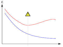

Now, a second problem with overfitting is described: unreliable model interpretation. Predictive modeling algorithms find variables that associate or correlate with the target variable. When models are overfit, the algorithm has latched onto variables that it finds to be strongly associated with the target variable, but these relationships are not repeatable. The problem is that these variables that appear to be strongly associated with the target are not necessarily related at all to the target. When we interpret what the model is telling us, we therefore glean the wrong insights, and these insights can be difficult to shed once we rebuild models to simplify them and avoid overfitting.
Consider an example from the 1998 KDD Cup data. One variable, RFA_3, has 70 levels (71 if we include the missing values), a case of a high-cardinality input variable. A decision tree may try to group all levels with the highest association with the target variable, TARGET_B, a categorical variable with labels 0 for non-responders and 1 for responders to a mailing campaign.
RFA_3 turns out to be one of the top predictors when building decision trees. The decision tree may try to group all levels with high average rates of TARGET_B equal to 1. The table below shows the 10 highest rates along with the counts for how many records match each value of RFA_3. The question is this: when a value like L4G matches only 10 records, one of which is a responder (10% response rate), do we believe it? How sure are we that the measured 10% rate in our sample is reproducible for the next 10 values of L4G?
We can gain some insight by applying a simple statistical test, like a binomial distribution test you can find online. The upper and lower bounds of the measured rate given the sample size is shown in the table as well. For L4G, we are 95% sure from the statistical test that L4G will have a rate between 0% and 28.6%. This means the 10% rate we measured in the small sample size could really in the long run be 1%. Or, it could be 20%. We just don’t know.
|
RFA_3
|
Count
|
TARGET_B = 1 Percent
|
Confidence Interval Lower Bound
|
Confidence Interval Upper Bound
|
95% Confidence above average
|
|
A2C
|
1
|
100.0%
|
No
|
||
|
S4B
|
2
|
50.0%
|
No
|
||
|
S4C
|
9
|
11.1%
|
0.0%
|
31.6%
|
No
|
|
L4G
|
10
|
10.0%
|
0.0%
|
28.6%
|
No
|
|
N1E
|
46
|
8.7%
|
0.6%
|
16.8%
|
No
|
|
S2D
|
200
|
11.0%
|
6.7%
|
15.3%
|
Yes
|
|
A4D
|
1,867
|
9.1%
|
7.8%
|
10.4%
|
Yes
|
|
S3D
|
1,989
|
9.4%
|
8.1%
|
10.7%
|
Yes
|
|
S3E
|
2,262
|
8.7%
|
7.5%
|
9.9%
|
Yes
|
|
S4D
|
2,675
|
9.6%
|
8.5%
|
10.7%
|
Yes
|
For the 1998 KDD Cup data, it turns out that RFA_3 isn’t one of the better predictors of TARGET_B; it only showed up as a significant predictor when overfitting reared it’s ugly head.
The solution? Beware of overfitting. For high-cardinality variables, apply a complexity penalty to reduce the likelihood of finding these low-count associations. For continuous variables, the problem exists as well and can be just as deceptive. For all problems you are solving, resample the data to assess models on held-out data (testing data), cross-validation, or bootstrap sampling.